vLLM metrics into VCF Operations, part 1: don't ship the histogram

vLLM’s /metrics endpoint is generous. Every model instance exposes a few hundred Prometheus series: counters, gauges, and — the problem — histograms with dozens of buckets each. Point a naïve scraper at it and push everything into VCF Operations and you get two things: a TSDB full of _bucket{le="0.05"} series nobody will ever graph, and a dashboard that tells an operator nothing.

This two-parter is the pipeline that fixed that. Part 1 is the design: what to compute, what to drop, and why. Part 2 is the operations story — scheduling, self-monitoring, alerts.

The core decision: percentiles are computed here, not there

A Prometheus histogram is a set of cumulative bucket counters:

vllm:time_to_first_token_seconds_bucket{le="0.1"}   1203
vllm:time_to_first_token_seconds_bucket{le="0.25"}  4871
vllm:time_to_first_token_seconds_bucket{le="0.5"}   7120
...
vllm:time_to_first_token_seconds_bucket{le="+Inf"}  7412
vllm:time_to_first_token_seconds_sum                1812.4
vllm:time_to_first_token_seconds_count              7412

Prometheus turns that into a P95 at query time with histogram_quantile. VCF Operations has no such function — it stores gauges. So the pipeline does the interpolation before pushing:

function Get-Percentile {
    param([array]$Buckets, [double]$Total, [double]$Percentile)
    $target = $Percentile * $Total
    $prevLe = 0.0; $prevCount = 0.0
    foreach ($b in $Buckets) {                    # sorted by le, +Inf last
        if ($b.Count -ge $target) {
            if ($b.Le -eq [double]::PositiveInfinity) { return $prevLe }
            $frac = ($target - $prevCount) / ($b.Count - $prevCount)
            return $prevLe + $frac * ($b.Le - $prevLe)   # linear within the bucket
        }
        $prevLe = $b.Le; $prevCount = $b.Count
    }
}

Linear interpolation within the bucket that crosses the target rank — the same approximation Prometheus makes. Out come four flat gauges per histogram: p50_ms, p95_ms, p99_ms, avg_ms (from _sum/_count). Twenty-odd series become four, and they’re the four an operator reads.

Applied to: TTFT, end-to-end latency, inter-token latency, time per output token, prefill time, decode time, inference time, queue time.

Rates need memory

Counters (generation_tokens_total, request_success_total) are useless as absolute values. What you want is tokens per second — which needs the previous sample. So the script is stateful: llm-metrics-state.json holds the last counters and timestamp per target, and each run computes deltas:

tokens_per_sec = (tokens_now - tokens_prev) / (t_now - t_prev)

Same trick, one step further, for live latency: _sum and _count are both counters, so Δsum / Δcount is the mean over the last interval — not the all-time mean the histogram gives you. That’s how you get live_avg_ttft_ms that reflects the last 60 seconds instead of the last fortnight.

Two guards make this safe:

• Stale-state protection. If the gap since the last run exceeds 300 s (scheduler stopped, server rebooted), the baseline is dropped rather than producing a diluted “per-second” rate averaged over an hour.
• Restart detection. A counter that went down means vLLM restarted; the delta is discarded for that cycle.

Derived metrics: what the raw numbers won’t tell you

Two computed values earn their place on the top of the dashboard.

Queue pressure ratio — (waiting + swapped) / (running + 1). Above 1.0 means more requests are waiting than being served: scale out.

System saturation score (0–100):

$saturation = ($kvCachePct * 0.5) + ($queuePressure * 25.0)
if ($saturation -gt 100) { $saturation = 100 }

Full KV cache alone scores 50; queue pressure of 2.0 scores the other 50. It’s a heuristic, and it’s deliberately one number: a dial that goes red when the engine is about to start swapping requests to CPU memory, which is the moment latency falls off a cliff. Warning at 75, critical at 90.

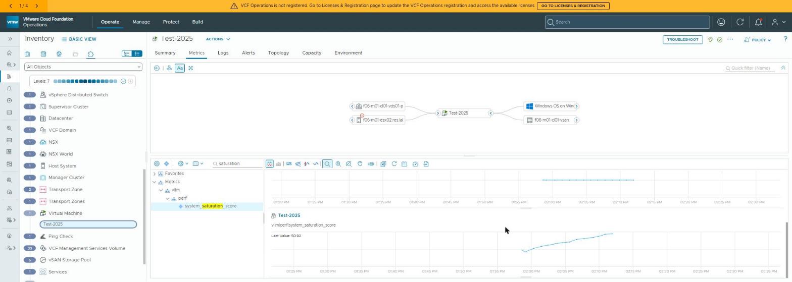The dial, as Ops draws it: one gauge climbing towards the warning line as KV-cache use and queue pressure rise together. (Test-mode data — see part 2.)

Also derived: prefix-cache hit rate (live and all-time), average request size from the dropped http_request_size_bytes _sum, uptime in days, and is_up = 1 on every successful scrape — so absence of the metric is the alert.

What gets dropped, and why

The $DropPrefixes list is as important as anything computed:

Everything that survives is truncated to two decimals before push — a small mercy for the TSDB.

The key hierarchy

Ops shows metrics as a tree, so the names are designed to browse:

vllm|system|is_up
vllm|throughput|total_tokens_per_sec
vllm|perf|live_avg_ttft_ms
vllm|perf|ttft|p95_ms
vllm|queue|pressure_ratio
vllm|memory|kv_cache_pct
vllm|cache|live_prefix_hit_rate_pct
vllm|process|rss_memory_gb

vllm | category | metric [| percentile]. An operator who has never seen vLLM can find “time to first token, 95th percentile” without a manual.

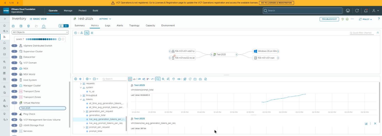
vllm | category | metric in the Ops metric picker — see part 2 for how this was captured.

Why this matters outside the lab

Organisations putting language models into service quickly discover that “is it up?” isn’t the question. The questions are: how long are users waiting for the first word, is the service about to run out of memory, and do we need another GPU before Friday? This pipeline answers them inside the same VCF Operations console the infrastructure team already lives in, so AI services get the same capacity planning, alerting and dashboards as everything else — no second monitoring stack, no new team to staff it.

Rules learned

• Never push raw histogram buckets into a gauge-oriented TSDB. Interpolate P50/P95/P99 client-side and push four gauges.
• Counters need state: keep the last sample, compute deltas, and drop the baseline after a long gap (300 s) rather than dilute the rate.
• Δsum/Δcount gives you live mean latency — far more useful than the all-time mean.
• One derived saturation score beats six raw gauges on the top of a dashboard. Make it explainable (KV% × 0.5 + pressure × 25).
• The drop-list is a design artefact, not housekeeping. request_params_* alone can double your series count.
• Name for browsing: product | category | metric.

Part 2: running it as a service, monitoring the monitor, and the four alerts.

Lab environment; opinions my own. Config shown is sanitised; the script’s test mode reads a local metrics file instead of a live endpoint.